Precision-Recall Curves 설명 및 그리기(구현)-Python
Goal
이 페이지에서는 Precision-Recall Curve가 무엇이고, 어떻게 그려지는지 알아보겠습니다. 이를 위해서 필요하다고 생각되는 Precision과 Recall, 그리고 Threshold와 Precision,Recall의 관계를 먼저 알아보겠습니다.
Precision(정밀도)과 Recall(재현율)
Precision과 Recall은 분류기의 모델을 평가하는 metric 입니다. Precision과 Recall은 Confusion Matrix를 기반으로 만들어집니다. Confusion Matrix는 분류 문제에서 모델이 예측한 것과 실제 Label과 일치, 불일치 하는 수를 요소로 가지며, 다음과 같습니다. Precision과 Recall외에도 Accuracy F1-score 등 여러가지 Metric도 Confusion Matrix를 기반으로 합니다.
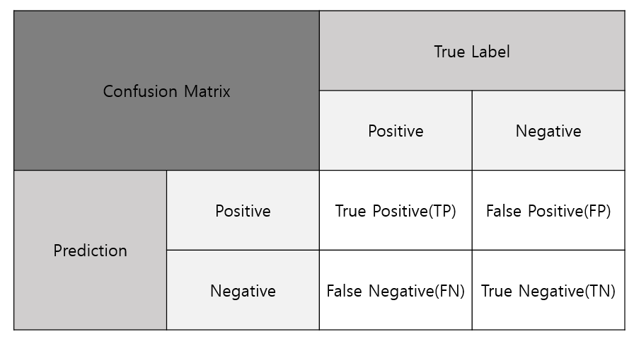
Confision Matrix에 있는 각 요소 들에 설명을 하겠습니다.
$TP$ = 실제 Positive를 모델이 Positive로 옳게 예측한 수
$TN$ = 실제 Negative를 모델이 Negative로 옳게 예측한 수
$FP$ = 실제 Negative를 모델이 Positive로 잘못 예측한 수
$FN$ = 실제 Positive를 모델이 Negative로 잘못 예측한 수
Precision과 Recall은 Confusion Matrix의 요소들로 다음과 같이 나타낼 수 있습니다.
- Precision은 모델이 Positive라고 예측한 것 중에서 실제로 Positive한 비율을 뜻하며, 다음과 같이 표현합니다.
- $Precision$ = $\cfrac{TP}{TP+FP}$
- Recall은 실제 Positive 에서 모델이 Positive라고 예측한 비율을 뜻하며, 다음과 같이 표현합니다.
- $Recall$ = $\cfrac{TP}{TP+FN}$
Threshold와 Precision, Recall의 관계
Positive / Negative를 확률로 구분하거나, 특정 Score로 구분하는 경우 Precision과 Recall은 Threshold의 함수입니다. 즉, Precision과 Recall은 Threshold 값에 따라 바뀌는 변수이며, 다음과 같이 볼 수 있습니다. (Threshold를 T로 줄이겠습니다.)
$Precision(T)$ = $\cfrac{TP(T)}{TP(T)+FP(T)}$
$Recall(T)$ = $\cfrac{TP(T)}{TP(T)+FN(T)}$
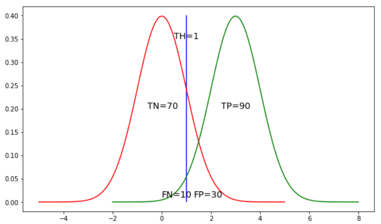
그림을 예를 들어 Threshold 값에 따른 Precision(T) 와 Recall(T)의 변화를 보겠습니다. 다음 그림은 T(=Threshold )가 1, 1.5, 2일 때의 Precision(T), Recall(T) 값입니다. 모델은 X축의 값이 Treshold 이상이면 Positive, Treshold 미만이면 Negative로 판단합니다.
1) T = 1
$Precision(1)$ = $\cfrac{TP(1)}{TP(1)+FP(1)}$
$Recall(1)$ = $\cfrac{TP(1)}{TP(1)+FN(1)}$
$Precision(1)$ = $\cfrac{90}{90+30}$ = 0.75
$Recall(1)$ = $\cfrac{90}{90+10}$ = 0.9
2) T = 1.5

$Precision(1.5)$ = $\cfrac{TP(1.5)}{TP(1.5)+FP(1.5)}$
$Recall(1.5)$ = $\cfrac{TP(1.5)}{TP(1.5)+FN(1.5)}$
$Precision(1.5)$ = $\cfrac{80}{80+20}$ = 0.8
$Recall(1.5)$ = $\cfrac{80}{80+20}$ = 0.8
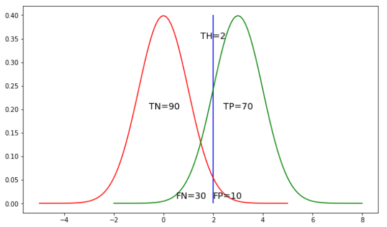
3) T = 2
$Precision(2)$ = $\cfrac{TP(2)}{TP(2)+FP(2)}$
$Recall(2)$ = $\cfrac{TP(2)}{TP(2)+FN(2)}$
$Precision(2)$ = $\cfrac{70}{70+10}$ = 0.875
$Recall(2)$ = $\cfrac{70}{70+30}$ = 0.7
즉, Precision과 Recall은 Threshold 값에 따라 바뀌는 변수임을 알 수 있습니다.
또한 Precision과 Recall 이 Trade-off 관계임을 알 수 있습니다.
Precision-Recall Curve Plot
Precision-Recall Curve 설명 및 특징
Precision-Recall Curves는 Parameter인 Threshold를 변화시키면서 Precision과 Recall을 Plot 한 Curve입니다. Precision-Recall Curves는 X축으로는 Recall을, Y축으로는 Precision을 가집니다. Precision-Recall Curve는 단조함수가 아닙니다. 이러한 이유로 ROC Curve보다 직관적이지 못하다는 단점을 가집니다.
Precision-Recall Curve Plot Algorithm
Precision-Recall Curve를 구체적으로 plot 하는 방법을 알아보겠습니다.
1. Probabillity (혹은 Score)를 기준으로 내림차순 정렬합니다.
2. Threshold를 가장 높은 Probability(or Scroe)로 정합니다.
3. Threshold 값에 따른 Model의 예측 값을 정합니다.
Threshold이상의 값이면 Positive, 미만이면 Negative로 예측합니다.
4. Recall과 Precision을 구해 Precision-Recall Curve에 Plot 합니다.
5. Threshold를 현재 Probability(or Scroe) 보다 한 단계 낮은 값으로 정하고 3번으로 돌아갑니다.
현재 Threshold보다 낮은 Probaility(or Scroe)가 없다면 종료합니다.
Precision-Recall Curve Plot Example
다음은 위의 과정을 설명하기 위한 예시입니다. True Label에 Positive, Negative가 각각 10개씩 있습니다.
1. Probability를 기준으로 내림차순으로 정렬합니다.
2. Threshold를 가장 높은 Probability인 0.9로 정합니다.
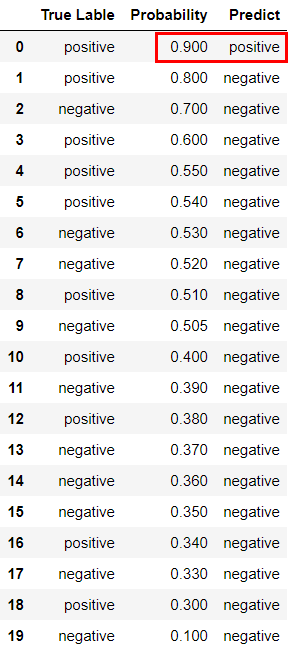
3. Threshold값에 따른 Model의 예측값을 정합니다. (현재 TH=0.9)
Probability >= Threshold이면 Positive로 Predict 합니다.
Probability < Threshold이면 Negative로 Predict 합니다.
4. Precision과 Recall 값을 구해 Precision-Recall Curve에 Plot합니다.
$Recall$ = 실제 Positive를 Positive로 예측 / 실제 Positive
$Precision$ = Positive로 예측한 것이 실제 Positive / Positive로 예측
Recall = $\cfrac{1}{10}$ = 0.1
Precision = $\cfrac{1}{1}$ = 1
Plot ( 0.1, 1 )
5. Threshold를 현재 Probability보다 한 단계 낮은 값으로 정하고 3번으로 돌아갑니다. Threshold = 0.8
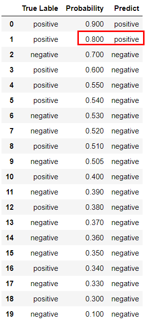
3. Threshold값에 따른 Model의 예측값을 정합니다. (현재 TH=0.8)
Probability >= Threshold이면 Positive로 Predict 합니다.
Probability < Threshold이면 Negative로 Predict 합니다.
4. Precision과 Recall 값을 구해 Precision-Recall Curve에 Plot합니다.
$Recall$ = 실제 Positive를 Positive로 예측 / 실제 Positive
$Precision$ = Positive로 예측한 것이 실제 Positive / Positive로 예측
Recall = $\cfrac{2}{10}$ = 0.2
Precision = $\cfrac{2}{2}$ = 1
Plot ( 0.2 ,1 )
5. Threshold를 현재 Probability보다 한 단계 낮은 값으로 정하고 3번으로 돌아갑니다. Threshold = 0.7

3. Threshold값에 따른 Model의 예측값을 정합니다. (현재 TH=0.7)
Probability >= Threshold이면 Positive로 Predict 합니다.
Probability < Threshold이면 Negative로 Predict 합니다.
4. Precision과 Recall 값을 구해 Precision-Recall Curve에 Plot합니다.
$Recall$ = 실제 Positive를 Positive로 예측 / 실제 Positive
$Precision$ = Positive로 예측한 것이 실제 Positive / Positive로 예측
Recall = $\cfrac{2}{10}$ = 0.2
Precision = $\cfrac{2}{3}$ = 0.67
Plot ( 0.2, 0.67 )
5. Threshold를 현재 Probability보다 한 단계 낮은 값으로 정하고 3번으로 돌아갑니다. Threshold = 0.6
이러한 과정을 반복하여 Threshold = 0.1까지 진행합니다.
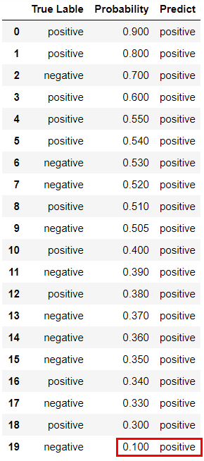
3. Threshold값에 따른 Model의 예측값을 정합니다. (현재 TH=0.1)
Probability >= Threshold이면 Positive로 Predict
Probability < Threshold이면 Negative로 Predict 합니다.
4. Precision과 Recall 값을 구해 Precision-Recall Curve에 Plot합니다.
$Recall$ = 실제 Positive를 Positive로 예측 / 실제 Positive
$Precision$ = Positive로 예측한 것이 실제 Positive / Positive로 예측
Recall = $\cfrac{10}{10}$ = 1
Precision = $\cfrac{10}{20}$ = 0.5
Plot ( 1 , 0.5 )
5. 현재 Threshold보다 낮은 Probaility(or Scroe)가 없어 종료합니다.
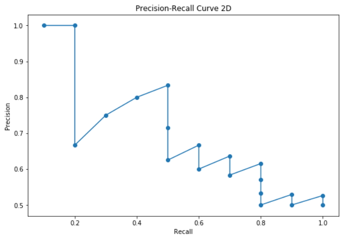
위의 과정 중에 나온 Recall, Precision 을 Plot하면 다음과 같은 Precision-Recall Curve가 그려지게 됩니다.
Code 구현
y_true = np.array([1,1,0,1,1,1,0,0,1,0,1,0,1,0,0,0,1,0,1,0])
y_scores = np.array([0.9,0.8,0.7,0.6,0.55,0.54,0.53,0.52,0.51,0.505,0.4,0.39,0.38,0.37,0.36,0.35,0.34,0.33,0.3,0.1 ])
def get_recall(y_true,y_scores,threshold):
predict_positive_num = len(y_scores[y_scores >= threshold])
tp = len( [x for x in y_true[:predict_positive_num] if x == 1] )
ground_truth = len(y_true[y_true==1])
recall = tp / ground_truth
return recall
def get_precision(y_true,y_scores,threshold):
predict_positive_num = len(y_scores[y_scores >= threshold])
tp = len( [x for x in y_true[:predict_positive_num] if x == 1] )
fp = len( [x for x in y_true[:predict_positive_num] if x == 0] )
precision = tp / (tp + fp)
return precision
def recall_precision_plot(y_true, y_scores):
recall, precision = [] , []
for _ in y_scores: # y_scores 를 thresholds 처럼 사용했음
recall.append(get_recall(y_true, y_scores, _ ))
precision.append(get_precision(y_true,y_scores,_))
fig = plt.figure(figsize=(9, 6))
#3d container
ax = plt.axes(projection = '3d')
#3d scatter plot
ax.plot3D(recall, y_scores, precision)
ax.scatter3D(recall,y_scores,precision)
#give labels
ax.set_xlabel('Recall')
ax.set_ylabel('Thresholds')
ax.set_zlabel('Precision')
ax.set_title('Precision-Recall Curve 3D')
plt.show()
fig = plt.figure(figsize = (9,6))
plt.plot(recall, precision)
plt.scatter(recall,precision)
plt.xlabel('Recall')
plt.ylabel('Precision')
plt.title('Precision-Recall Curve 2D')
plt.show()
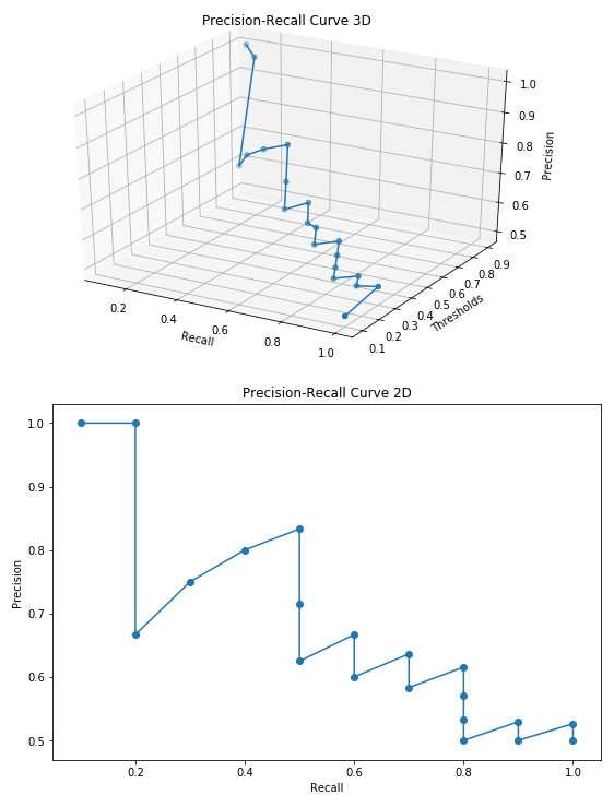
recall_precision_plot(y_true,y_scores)코드 결과물 및 설명
우리가 보통 보는 Precision-Recall Curve는 Precision과 Recall 축으로만 구성된 2D Curve입니다. 하지만, Precision과 Recall은 Parameter인 Threshold에 따라 정해지는 값이므로, Threshold까지 포함하면 3D가 됩니다. 이를 표현하기 위해 Threshold 축을 추가하여 3D로 그려봤습니다. 이 3D에서 Precision-Recall 평면으로 Projection하면 우리가 평소에 보던 2D Curve를 볼 수 있습니다.
이번 포스팅에서는 Precision-Recall Curve 에 대해 알아봤는데 이와 성격이 비슷한 ROC Curve 설명 및 그리기는 다음 URL에 정리해두었습니다.
https://ardentdays.tistory.com/21
ROC Curve 설명(해석) 및 그리기(Python)
ROC Curve 설명(해석) 및 그리기(Python) Goal 이 페이지에서는 ROC Curve가 무엇이고, 구체적으로 어떻게 그리는지 알아보겠습니다. 그동안 ROC Curve에 대해서 알고있던 것들은 분류기(classifier)에 쓰이는 M
ardentdays.tistory.com
'인공지능 > ML' 카테고리의 다른 글
| Isolation Forests for Outlier Detection (0) | 2021.04.30 |
|---|---|
| ROC Curve 설명(해석) 및 그리기(구현)-Python (2) | 2021.02.28 |
| 이상치 감지를 위한 Depth-Based Method (0) | 2021.02.25 |
| Box plot 정리 (0) | 2021.02.25 |
| Stutent's t-distribution ( t분포) (0) | 2021.02.25 |